Quick Start

Author:Kyle M. Douglass Contact:kyle.m.douglass@gmail.com organization:École Polytechnique Fédérale de Lausanne (EPFL) revision:Revision: 3 date:2016-11-06 abstract:This quick start guide shows how to get up and running with B-Store as quickly as possible.

Table of Contents

• Quick Start
  • Installation
    • Anaconda
    • Installation from Source
  • Getting Started
    • Background
    • Jupyter Notebook Examples
    • B-Store Test Datasets
    • Workflow Summary
  • Build a HDF Datastore with the GUI
    • Misc. Build Options
  • Programming with B-Store
    • Parsing Files to assign Dataset IDs
    • Building a Datastore
    • Batch Analysis from a B-Store Database
  • Getting Help

Installation

Anaconda

Installation is most easily performed using the Anaconda package manager. Download Anaconda for Python 3 (or Miniconda) and run the following commands in the Anaconda shell:

conda update conda
conda config --append channels soft-matter
conda create -n bstore -c kmdouglass bstore

The above commands add a custom channel to the package manager (soft-matter) and give it lower priority over the default channel. Then, a new conda environment named bstore is created and the bstore package is installed from the kmdouglass channel.

If you would like to use Jupyter Notebooks–which aren’t required–, then be sure to run these commands after installing B-Store:

conda install jupyter nb_conda

Every time you want to run bstore, ensure that you are working in the bstore environment with

activate bstore

on Windows and

source activate bstore

on Linux and Mac.

Installation from Source

Alternatively, the source code for B-Store may be cloned from https://github.com/kmdouglass/bstore/. A list of dependencies may be found inside the requirements.txt file inside the repository.

The master branch contains code that has been more thoroughly tested than any other branch. The development branch contains the version of the code with the latest features but is more likely to suffer from bugs.

Getting Started

Background

The B-Store workflow is divided between these two tasks:

1. Sort and place all the files from a single molecule localization microscopy (SMLM) acquisition into a single file known as a Datastore.
2. Automatically access this datastore for batch analyses.

B-Store uses popular scientific Python libraries for working with SMLM data. Most notably, it uses Pandas DataFrames for working with tabulated localization data and the standard json module for handling metadata. Images are treated as NumPy arrays whose image metadata can be read from tiff tags (OME-XML and Micro-Manager metadata are currently supported). Reading and writing from/to HDF files is performed with h5py (though Pandas uses PyTables for a few operations).

What all this means is that if you can’t do something with B-Store, chances are you can implement a custom solution using another Python library.

Jupyter Notebook Examples

If you want to learn more after working through the quick-start guide, then you can find examples inside the Jupyter Notebooks at the B-Store GitHub repository.

Jupyter Notebooks are a great way to interactively work with B-Store when writing code and are very common in the scientific Python community. They are free, powerful, and provide a convenient way to document your work and share it with others. Alternatively, you may use any other Python interpreter to work with B-Store functions.

B-Store Test Datasets

The B-Store test files repository contains a number of datasets for B-Store’s unit tests. These datasets may also be used to try out the code in the examples or in this guide.

Workflow Summary

B-Store is a collection of tools for working with SMLM data. You may interact with these tools in two different ways:

1. by using the GUI, and
2. by writing Python code

Once you have a set of HDF files, you may open them in any software package or language that supports HDF, such as MATLAB.

Build a HDF Datastore with the GUI

To start the GUI, navigate to the console window (or Anaconda prompt). If you installed B-Store from Anaconda, be sure to activate the bstore environment using whatever name you chose when creating it:

source activate bstore

If you’re on Windows, don’t use the word source.

Once activated, simply run the program by typing:

bstore

In the window that appears, select File > New HDF Datastore.... The following new dialog will appear:

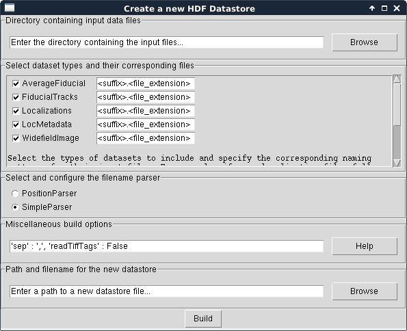
First, choose the directory where the raw data files and subdirectories are located. We will use the test files for the SimpleParser for this example. Please note that this directory and all of its subdirectories will be searched for files ending in the suffix.filename_extension pattern specified in the next field.

Next, select what types of datasets should be included in the datastore. For this example, check Localizations, LocMetadata, and WidefieldImage and uncheck the rest. Set the filename extension of Localizations, LocMetadata, and WidefieldImage to .csv, .txt, and .tif, respectively. This will tell the build routine what files correspond to which types of datasets.

If your files have a special identifier in their filename, like locs for localizations, you can enter search patterns like locs*.csv. The asterik (*) will act as a wildcard such that files like cells_locs_2.csv or Cos7_alexa647_locs.csv would be found during the file search.

Leave the parser set to SimpleParser. A parser converts a filename into a set of DatasetIDs that will uniquely identify it inside the Datastore.

After this, leave the Misc. options as they are. This box allows you to manually specify options for reading the raw data files. ‘sep’ for example is the separator between columns in a .csv file. If you have a tab-separated file, change ‘,’ to ‘t’ (t is the tab character). Change ‘readTiffTags’ from False to True if you have Micro-Manager or OME-XML metadata in your tif image files. Please note that this may fail if the metadata does not match the filename like, for example, what would happen if someone renamed the file.

Finally, use the Browse dialog to select the name and location of the HDF datastore file in the top-most field.

The window should now look like this:

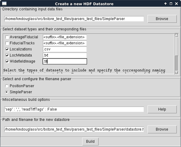
Click the Build button and when it completes, you should have a nice, new HDF Datastore with your data files structured safely inside it.

Misc. Build Options

The misc. build options, like sep and readTiffTags, are passed to each Dataset’s method for reading data from files. They are specified in the same notation as Python dictionaries except they omit the curly braces. Each one is optional, so you need not specify any of them.

The name of each option must be surrounded in single quotation marks. The value for each option is a Python datatype and is separated from the option’s name by colon. All option/value pairs are separated by commas. True and False are case-sensitive. Strings are also surrounded by single quotes.

The current list of options is:

1. sep - The column separator in the raw text csv files. Common values include commas ‘,’ and tabs ‘\t’.
2. readTiffTags - Determines whether tif image metadata should be read and recorded in the HDF datastore. Accepts either True or False. Note that this may fail to read the tif images if the filename does not match the metadata.

For Pythonistas: The evaluation of the string inside this Entry is

performed with ast.literal_eval(). It is a secure method, unlike eval(), but can only evaluate basic Python datatypes.

Programming with B-Store

B-Store also has an API which allows you to write scripts and Python code to integrate B-Store into your custom workflows.

Parsing Files to assign Dataset IDs

A B-Store Datastore is a storage container for things like sets of localizations, widefield images, and acquisition metadata. Each dataset in the datastore is given a unique ID. A parser reads your data from files and gives it a meaningful set of datastore IDs. For example, if you have localizations stored in a comma-separated text file named HeLaL_Control_1.csv and you use the built-in SimpleParser, then your dataset will have the following ID’s:

1. prefix - ‘HeLaL_Control’
2. acqID - 1

You can follow along by entering the following code into the Python interpreter of your choice and using the SimpleParser test files.:

>>> import bstore.parsers as parsers
>>> sp = parsers.SimpleParser()
>>> sp.parseFilename('HeLaL_Control_1.csv', 'Localizations')
>>> sp.dataset.datasetIDs
{'acqID': 1, 'prefix': 'HeLaL_Control_1'}

Here, Localizations refers to a specific dataset type used by B-Store to read and write localization data.

B-Store comes with two built-in parsers: SimpleParser and PositionParser. The SimpleParser can read files that follow the format prefix_acqID.(filename extension). The very last item of the filename is separated from the rest by an underscore and is always assumed to be an integer. The first part of the filename is a descriptive name given to the dataset.

The PositionParser is slightly more complicated, but gives you greater flexibility over how your filenames are read. It assumes that each dataset ID is separated by the same character(s), such as _ or -. You then specify the integer position (starting from zero!) that each ID is found in.

For example, say you have a filename like HeLa_Data_3_2016-05-12.csv. You want HeLa to be the prefix, Data to be ignored (not used to assign an ID), 3 to be the acquisition ID number, and 2016-05-12 to be the date. These correspond to positions 0, 1, 2, and 3 in the filename, respectively, and the separator is an underscore (_). You would initialize the PositionParser like this:

>>> pp = parsers.PositionParser(positionIDs = {
>>>     0 : 'prefix', 2 : 'acqID', 3 : 'dateID'})

Changing the separator of ‘positions’ is also easy: simply specify a sep parameter to the PositionParser’s constructor. We can change the seperator to hyphen underscore (-_) like this:

>>> pp = parsers.PositionParser(
>>>>    positionIDs = {
>>>         0 : 'prefix', 2 : 'acqID', 3 : 'dateID'},
>>>     sep = '-_')

If you require a customized parser to assign ID’s, the Jupyter Notebook tutorial on writing custom parsers is a good place to look.

Building a Datastore

You will typically not need to work directly with a parser. Instead, the B-Store datastore will use a specified parser to automatically read your files, assign the proper ID’s, and then insert the data into the database.

Let’s say you have data from an experiment that can be parsed using the SimpleParser. (Test data for this example may be found at https://github.com/kmdouglass/bstore_test_files/tree/master/parsers_test_files/SimpleParser .) First, we setup the parser and choose the directory containing files and subdirectories of acquisition data.:

>>> from bstore import database, parsers
>>> from pathlib import Path
>>> dataDirectory = Path('bstore_test_files/parsers_test_files/SimpleParser')
>>> parser = parsers.SimpleParser()

Next, we create a name for the HDF file that a HDFDatastore points to. The HDFDatastore class will be used to interact with and create B-Store databases.:

>>> dsName = 'myFirstDatastore.h5'

After this, we tell B-Store what types of files it should know how to process:

>>> import bstore.config as cfg
>>> cfg.__Registered_DatasetTypes__ = [
        'Localizations', 'LocMetadata', 'WidefieldImage']

Localizations, LocMetadata, and WidefieldImage are built-in dataset types. Telling B-Store what types of files to look for helps prevent it from mistakenly thinking a random file that accidentally entered the directory tree contains SMLM data.

Finally, we create the database by sending the parser, the parent directory of the data files, and a dictionary telling the parser how to find localization files to the build method of myDS. Note that myDS must be created inside a with...as... block to ensure the file is properly opened and closed. The put() and build() methods of HDFDatastore both require the use of with...as... blocks; all other methods do not.:

>>> with database.HDFDatastore(dsName) as myDS:
>>>     myDS.build(sp, dataDirectory, {'Localizations'  : '.csv',
                                       'LocMetadata'    : '.txt',
                                       'WidefieldImage' : '.tif'})
6 files were successfully parsed.

This creates a file named myFirstDatabase.h5 that contains the 6 datasets contained in the raw data. (If you want to investigate the contents of the HDF file, we recommend the HDFView utility.)

To specify exactly how data is read from your raw files, please see Tutorial 4 in the examples. This will teach you how to user Readers to read data in custom file types into Python and subsequently place them inside the HDFDatastore.

Batch Analysis from a B-Store Database

Another great utility of the B-Store database is that it enables batch analyses of experiments containing a large number of acquisitions containing related but different files.

As an example, let’s say you want to extract all the localization files inside the database we just created and filter out localizations with precisions that are greater than 15 nm and loglikelihoods that are greater than 250. We do this by first building an analysis pipeline containing processors to apply in sequence to the data.:

>>> from bstore import batch, processors
>>> uncertaintyFilter = processors.Filter('uncertainty', '<', 15)
>>> llhFilter = processors.Filter('loglikelihood', '<=', 250)
>>> pipeline = [uncertaintyFilter, llhFilter]

Next, use an HDFBatchProcessor to access the database, pull out all localization files, and apply the filters. The results are saved as .csv files for later use and analysis.:

>>> bp = batch.HDFBatchProcessor(dsName, pipeline)
>>> bp.go()
Output directory does not exist. Creating it...
Created folder /home/douglass/src/processed_data

Inside each of the resulting subfolders you will see a .csv file containing the filterd localization data. A more complete tutorial may be found at https://github.com/kmdouglass/bstore/blob/master/examples/Tutorial%202%20-%20Introduction%20to%20batch%20processing.ipynb .

Getting Help

If you have any questions, feel free to post them to the Google Groups discussion board: https://groups.google.com/forum/#!forum/b-store

Bug reports may made on the GitHub issue tracker: https://github.com/kmdouglass/bstore/issues